How to split and extract text from data columns in Excel & Google Sheets

Sometimes, your data comes with several pieces of information in one column. Like a column with U.S. states in the format US-TX. Or a column with companies and the product they sell.

But say you want country (US) separate from state (TX). Good thing there are easy ways to separate data points into two or more columns.

I’ll show two ways to create multiple new columns out of one old column. We’ll use Google Sheets — but the same tricks should work with LibreOffice Calc, Excel, or any other spreadsheet software.

The first method is the formula =SPLIT():

1st method

Split columns with SPLIT()

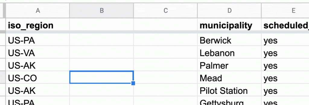
1. Create at least two new columns next to the column whose data you want to split. To do so, click on the header (A, B, C, etc.). Then click the little triangle and select “Insert 1 right.” Repeat to create a second empty column.
2. In the first empty column, write =SPLIT(B1,"-"), with B1 being the cell you want to split and - the character you want the cell to split on. (If you see the error #REF! in your cell, you’ll need to create more columns.)
3. To apply the changes to the cells below, drag down the blue square in the bottom right of the selected cell(s). Double-click on the blue square to fill all remaining cells.

2nd method

Extract content from columns with LEFT()

Sometimes you don’t have clear separator characters, but just want to extract the first or last characters of a cell. To do so, use the formulas =LEFT(B1,2), =RIGHT(B1,8), and =MID(B1,2,4):

1. Insert a new column. (Or two. Or three! As many as you need.)
2. In the new column(s), write
   =LEFT(B1,2) to extract the first 2 characters of the cell B1.
   =RIGHT(B1,8) to extract the last 8 characters of the cell B1.
   =MID(B1,4,2) to extract the 2 characters following the 4th character in B1.
3. To apply the changes to the cells below, drag down the blue square.